An introduction to the theory of operation
Pulse-passing transformers are analogous in many respects with wide band transformers for sinusoidal working, inasmuch as the pulse may be analysed into a Fourier spectrum the components of which bear certain phase relationships.
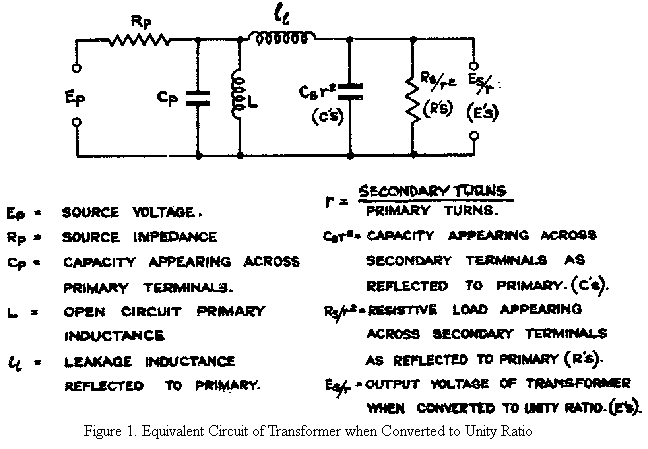
Thus, pulse-passing transformers require to possess a controlled frequency characteristic, but unlike wide band transformers, the phase relationships must be considered. A simple approximate equivalent circuit of a transformer is shown in Fig. 1. Loss resistances are not shown and will be considered separately.
Now it is well known that when such a transformer is used for wide band working, it may be simplified to two equivalences which are applicable at the lower and upper limits of the frequency spectrum as illustrated in Figs. 2 and 3 respectively.
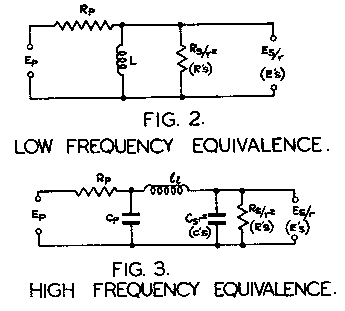
From Fig. 2, the output at low frequencies is given by
E's = Ep (R'S/Rp+R'S) • (jωL/RT + jωL),
where RT is the parallel value of Rp and R'S (i.e., the total load reflected in shunt with the primary winding).
For impulse working, this equation is best stated in operational form as
E's = Ep (R'S/Rp+R'S) • (pL/RT + pL) [Ep],
and has a solution
E's = Ep (R'S/Rp+R'S) exp. (- (RT T)/L), where T is the pulse duration.
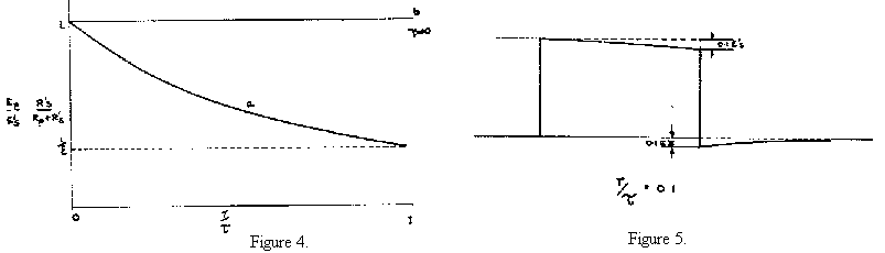
Thus the application of a rectangular pulse will, due to finite low frequency response (or time constant τ = L/RT ) give rise to the response of Fig. 4 where the instant of application of the pulse is at T/τ = 0 and the difference between curves (a) and (b) shows the resulting droop of the pulse from its initial value. Fig. 5 shows the typical distortion of a pulse of duration T = 0.1 τ. It is seen that a droop of 10% of the initial value occurs during the pulse and that a 10% overshoot exists when the pulse ends. Thus, summarising, it is seen that this form of pulse distortion is controllable by the ratio of L/RT to the pulse duration, and this ratio should be large to achieve faithful reproduction.
As in transformers for wide band working, the equivalence of Fig. 3 may be considered to have an independent influence on the high frequency response, or in pulse transformers on the characteristics of the leading and trailing edges of the pulse.
The equivalent circuit of Fig. 3 yields a third order differential equation, and the treatment of the mathematics is beyond the scope of this paper but may be referred to in TRE Monograph 5A. It will be sufficient to say here that where either Cp or C'S is negligible, the equation reduces to a second order type and a simple graphical solution is available for computing the response. The leakage inductance circuit may, approximately speaking, distort the leading edge in two ways:- It may introduce a time delay followed by an oscillatory waveform as shown in Fig. 6, where this new pulse distortion is superposed on that already existing due to limited low frequency response as shown in Fig. 5. Alternatively, the leading and trailing edges may reach their final values exponentially when the circuit is critically damped (Fig.7).
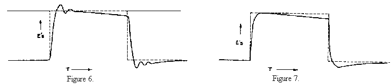
Figs. 6 and 7 exemplify the typical transformer responses encountered, and much of the art of design lies in the accurate control and minimising of such distortion.
Returning again to wide band transformers, it is known that primary inductance is a function of frequency, and the question therefore arises as to what value of primary inductance is relevant in a pulse transformer.
Two factors combine in influencing the permeability of the core material upon which inductance depends; these are core polarisation, (peculiar to pulse transformers only), and eddy currents in the laminations which account for the dependence of inductance upon frequency mentioned above.
In connection with the first of these factors, imagine that the waveform of Fig. 8A, which represents a repetitive series of pulses of duration t spaced in time by an interval T much greater than t, is applied to the primary of a transformer having no secondary loads.
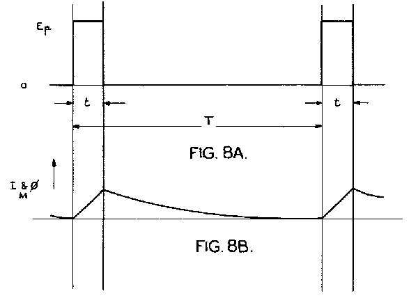
Let the source impedance be such that the primary time constant is much greater than t but much less than T. Then the primary voltage will be substantially rectangular throughout the pulse and
EP = dØ/dt × Np ×10-8 where Np is the number
of primary turns. This relationship shows that the core flux will increase linearly with time during the pulse. If the laminations be supposed so thin that eddy losses are negligible, the magnetising current will rise linearly with time, provided the permeability is constant. Thus the magnetising current IM, and Ø the core flux, rise as shown at Fig. 8B. Between the pulses, since the transformer time constant is much less than T, IM will fall to zero. Now since IM is a measure of H, (the MMF applied to the core), and further, since this has an excursion from 0 to HT where HT is the value of H at the end of any pulse, it follows that the B.H. operating loop will lie asymmetrically to the origin on the axis of B and H and thus the core will behave as though polarised to a steady value of HT/2. This is illustrated in Fig. 9 which shows the B.H. minor loop of an actual transformer. The polarisation discussed above results in rather low values of permeability, and saturation occurs at relatively low values of AN, AB,being the change of flux density during the pulse.
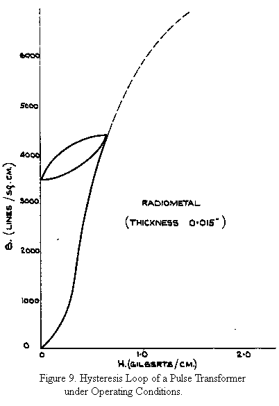
As an example, mumetal at a working value of ΔB = 600 lines/sq. cm. gives a permeability of 5000, and saturates at about 1500 lines/sq. cm.
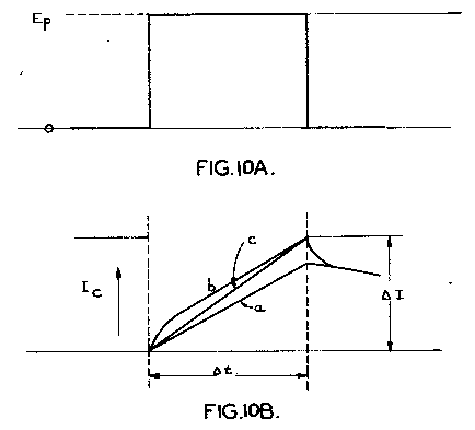
Coming now to the second factor causing a reduction in permeability, we have eddy current loss. On application of a pulse, immediate penetration of the flux into the core is prevented by skin effect, so that at this instant the rate of growth of magnetising current is high. This is illustrated in Fig. 10 where A of, the figure shows the pulse to an enlarged time scale, and B of the figure in curve (a) illustrates the growth of magnetising current in the absence of skin effect and (b) with skin effect. During the curved portion of (b), the flux penetration is taking place, and when it is complete, curves (a) and (b) become parallel. The displacement between the curves represents the eddy current loss, which becomes constant when the curves are parallel.
Inductance is defined fundamentally as
L = -E/(di/dt)
where E is the voltage produced across the inductance by the rate of growth of current. In dealing with pulse transformers it is convenient to introduce an apparent inductance,
L = Ep/(ΔI/Δt)
and here the primary voltage gives rise to an average rate of change of current as shown by curve (c), having the same final value as curve (b) of Fig. 10B. This will not be pursued further here, except to state that this apparent inductance relates to an apparent permeability which may be plotted as a function of pulse duration; in this form, it is of the greatest convenience to designers, as it permits the loss current to be controlled in terms of core material, lamination thickness, physical size and primary turns.
We have seen that in order to avoid pulse droop, the time constant L/RT is made much greater than the pulse duration. It would be better to re-define this time constant L/RT (i.e., we use the apparent primary inductance), but in any event the droop is not exponential in form as the inductance is not constant throughout the pulse.
For the example already quoted, namely mumetal, and using a lamination thickness of 0.004 in., the apparent permeability for 1 µsec pulse working is 740, and at 20 µsec it is 3000.
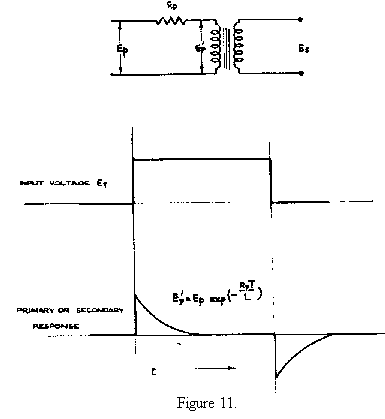
It is often of value to differentiate the pulse in a manner analogous to capacity-resistance network differentiation. Pulse transformers may be made to do this, and a special design has been developed for the production of time constants from ½ to 40 µsec. Such differentiating transformers have gapped cores, and this results in a sensibly constant value of inductance throughout the pulse, so that the waveform delivered is exponential. The circuit and typical waveforms are shown in Fig. 11.
Applications of Pulse Transformers
The advent of the pulse transformer has greatly increased circuit flexibility and has often afforded considerable
economy in the use of valves.
Some of the more important uses of the device are listed below.
(a) Impedance matching,
(b) Pulse inversion,
(c) The generation of a pulse waveform in a floating winding,
(d) Voltage transformation,
(e) Current transformation,
(f) Differentiation.
(a) and (b) of the list need no comment - their usefulness is evident. Under (c) the fact that a transformer secondary is, in effect, a floating generator is of considerable value in circuit design.
Amplifying (d) and (e), one of the most important facilities offered by the transformer is the fact that the impedance characteristics of the source appear reflected to the secondary terminals.
Thus a transformer fed from a low impedance (constant voltage) source, such as a cathode follower, will deliver a constant secondary pulse voltage irrespective of load, up to the limit set by source overload. Droop due to core loss current will be negligible and the pulse will have a flat top, though the shape of the pulse edges will vary with load.
Conversely, a transformer fed from a high impedance (constant current source) such as a pentode, will deliver a constant current irrespective of secondary voltage demanded so long as the transformer losses are small. Again the pulse edges will be influenced by secondary loading.
Transformers falling within this second category have been used in automatic range tracking circuits.
Finally, differentiating transformers owe their superiority over capacity-resistance differentiation to the fact that impedance matching, pulse inversion, and "floating pulse" generation (as under (c)) are available simultaneously with the pulse shaping facility.