1. INTRODUCTION
The necessity for Radar trainers was discovered early in the history of radar, and from the early type of simple synthetic trainers has grown a design technique which now
involves the use of radar and radio circuitry, mechanical
devices, optical systems, and the techniques of
ultrasonics, etc. It is proposed in this article to deal
with the production and control of simulated displays, and the
control of moving synthetic targets, rather than with Radar
systems.
The production of the synthetic echo is usually a simple design problem, but the control of the synthetic display and of the synthetic target's movements is complex, particularly in the case of radar air interceptions, where both target and interceptor are in motion. In general, range, bearing and elevation are fundamental requirements, with amplitude of signal, signal/noise ratio, fading, ground or sea returns, IFF, etc. as requirements special to each radar system.
2. USE OF RADAR TRAINERS
The use of radar trainers in this War is far more wide
spread than is generally realised. It is estimated that
approximately 2000 synthetic radar trainers have been in
service since 1940, enabling the equivalent of a fleet of
4000 aircraft to be used for training purposes, representing
a total saving to this country of £56,000,000. Since the
beginning of the War 50,000 radar operators, controllers,
navigators etc, have received initial training on synthetic
radar trainers designed by TRE.
3. TARGET PULSE PRODUCTION
There are numerous well-known methods of obtaining
pulses of ½ to 20 μsecs. e.g. delay networks, differentiation
of square waves, damped ringing circuits, etc. Rounded
pulses, pulses with sharp leading edge, and triangular
pulses can be easily produced to simulate the shape of the
re-radiated target pulse.
A circuit which has been used is given below:-
(a) Thyratron Delay
Line Pulse
Producer
This circuit is
capable of producing
square pulses of
short duration (from
0.1 µsec. to 2 to 3µsec.) As shown,
the output is positive,
but by removing the
load resistance R to X,
negative pulses may
be obtained.
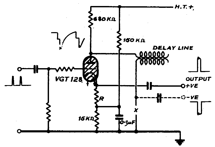
Fig. 1 Thyratron delay line pulse producer.
The delay line consists of two layers of close wound 40 SWG dsc wire on a 3/16" diameter core of PVC. The two layers are wound in opposite directions. The pulse width is proportional to the length of the line, being approximately 1 microsecond for each 3½ inches.
The thyratron is normally biassed so that no current flows and the anode voltage is that of the H.T. line. Application of a positive waveform to the grid causes the thyratron to conduct which effectively connects the charged artificial load consisting of the resistance R and the internal resistance of the valve. The artificial line discharges into this terminating resistance producing a square pulse. The output is taken across R which normally has a value of two or three hundred ohms. The amplitude of the output may be from 1 to 50 volts depending on R. The time of rise of the pulse is of the order 1/100 of µsec. and the time of fall 1/30 micro-second.
The circuit may be triggered from almost any waveform of sufficient amplitude; sinewaves, square waves from ranging circuits and positive pulses have all been used. The grid circuit constants depend on the triggering waveform.
4. DELAY CIRCUITS
A trainer usually needs to be locked from the main
equipment by a locking signal which may take several forms,
such as sine wave, square wave, pulse, sawtooth, etc. Delay
circuits which have been used are:-
(a) Synchronised from sine wave
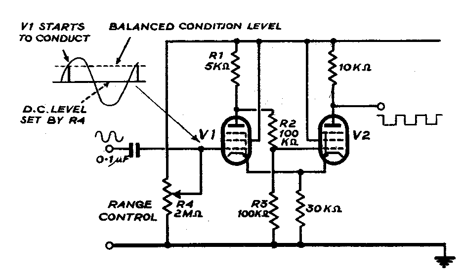
(i) Sine wave controlled long tail pair
Fig. 2 Sine wave input delay circuitIn this circuit (figure 2) a sine wave, superimposed on a variable D.C. bias obtained from a potentiometer across the H.T. supply, is fed to the grid of Vl. Due to the network R1, R2, R3, the grid potential of V2 is determined by the-anode potential of V1. When the voltage variation (D.C. input sine wave passes over the grid base of V1 a proportion of the anode coupled to the grid of V2) is fed back to V1 by means of the common cathode load. This positive feedback cuts V2 off for the duration of that part of the sine wave over which V1 is conducting. This portion is determined by the standing bias of Vl. For the remainder of the sine wave V1 is cut off. A square wave of steep edges is produced at the anode of V2 which may be differentiated and cut by a diode to produce a movable pulse locked to the sine wave.
(ii) The sine wave may also be squared and differentiated to produce a trigger for other delay circuits.
(b) Synchronised from a pulse
(i) Transitron Square Wave Generator ) These circuits
(ii) Kipp Relay and Multi-Vibrators ) are well known.
(iii) Phantastron
This circuit has proved one of the most flexible and satisfactory for use in radar trainer design, and it is used because of its high degree of linearity. This linearity, is essential where continuous calculators (described later) are used. No description is given as this circuit has been fully described in TRE Report T1316. Although the VR116 is usually recommended for this circuit, the more easily obtained VR91 has been successfully used. Where economy of valves is a consideration the grid diode may also be omitted with little loss of stability of delay time.
(iv) Sanatron
The Sanatron is a development of this circuit using two valves and is fully described in TRE Report T1469, This circuit has been used in AI trainers, where the total delay time is small.
(v) Triggered Delay Circuits
The trailing edge of the square wave obtained from both the sanatron and phantastron circuits may be locked from one of a series of calibration pips. Thus extremely stable delays variable in steps equal to the interval between the calibration pips may be obtained.
(c) Synchronised from a sawtooth
(i) Sawtooth controlled gas filled relay
A sawtooth time base waveform can be fed to the grid of the thyratron delay line pulse producer described in 3(a) and the bias on the thyratron can be set so that the relay will not strike until this voltage is exceeded by the sawtooth. Variation of the bias potential therefore provides variation of range.
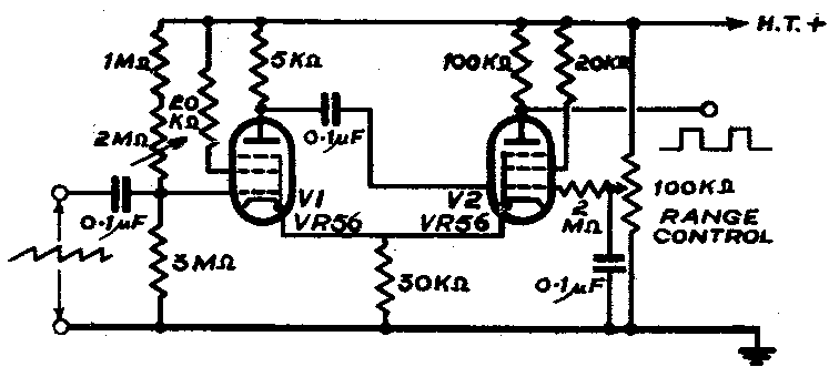
(ii) Sawtooth controlled long tail pair with feedback
Fig.3 Sawtooth input delay circuit
An extremely wide control of minimum to maximum range can be obtained by this method. (Fig.3) The time base waveform is fed to the grid of one of the valves in a long tail pair, the other grid potential being determined by the slider of a potentiometer across the E.H.T. line.When the first grid reaches the potential of the second, V1 takes current and the voltage drop of V1 is fed via the coupling condenser to the grid of V2 cutting this valve off. V2 remains cut-off until the first grid is brought sufficiently negative by the flyback of the sawtooth. A positive square wave, whose duration is determined by setting of the grid potential of V2, is obtained at the anode of V2.
(d) Synchronised from a square wave
(i) Condenser discharge method
Figure 4. Condenser discharge delay circuitA square wave (negative going) from a normal squared sine wave or other source is fed to one side of C1 (see the grid of V1, cutting this valve off. fig.4) from a variable tapping on the anode load.
The voltage drop is developed across R2 via C1 and fed to C1 now starts to discharge through R2 and R1 in series, until the grid potential of V1, is zero, when diode action of grid and cathode of V1 prevents the grid from becoming more positive. This produces a square wave at the determines the amplitude of square wave to Cl and therefore the amount by which the grid of V1 is taken anode of V1. The width is controlled by R1 which negative. By substituting a number of variable resistances giving an equivalent value to R1, the single square wave can control several pulses. The maximum width of the variable square wave is equal to the width of the input square wave. The circuit can also be operated from a large positive pulse as shown in dotted lines in the diagram (fig.4).
5. BEARING OR GATE CIRCUITS
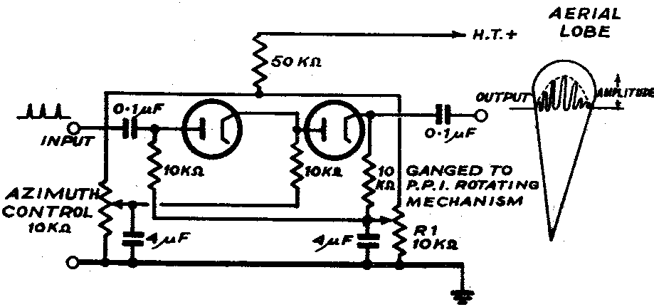
(a) D.C. Gate Circuit
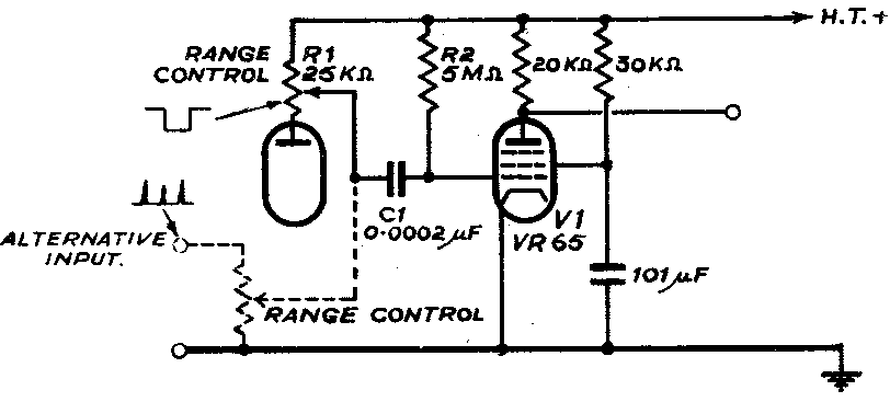
Fig.5 D.C. Gate Circuit
For simulation of radar systems using beam aerials on
PPI's (CHL/GCI etc.) a diode gate circuit shown in fig. 5
can be used to simulate the main lobe passing across the
target.
Signals are only passed when the diode biases are equal, one of the bias potentiometers being connected to the rotating aerial system, the other can be set manually or can be controlled for changes in bearing. The area on which the echo
can appear on the PPI is limited by a sector in which the
potentiometer arm moves over the gap in the winding.
The arc length in degrees = ![]() volts across Rl
angular length of potentiometer winding (approximately).
volts across Rl
angular length of potentiometer winding (approximately).
(b) 360° A.C. Gate Circuit
A system which avoids the blank area, inevitable in the
above D.C. system, is given below.
The control potentiometers in this case consist of a continuous toroidal resistance element having two tappings at right angles to one another and two sliders 180° apart. These potentiometers are described in detail in paragraph 5(e). The supply voltage to both the potentiometers is connected to the sliders as shown. The voltage waveform at one of the tappings as the potentiometer is rotated is a symmetrical triangle, the waveforms from two tappings of the same potentiometer being similar but 90° out of phase. If the sliders of one potentiometer are fixed and those of the other are rotated, there will be two positions where the voltages at one pair of corresponding taps are equal, and two positions where those at the other pair are equal, but at only one of these positions are both equal at the same time.
The voltages obtained from the corresponding pairs of tappings are used to operate two double diode gate circuits, there being but one position of the potentiometers where both are open together. The second gate may be considered a type of phase discriminator.
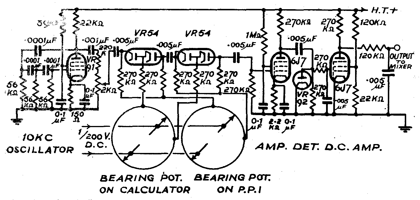
Fig.6 360° A.C. Gate Circuit
A sine wave of frequency 10 Kc/s is applied to the diode gates as shown. When both are open the waveform passed (which has been attenuated during its passage) is amplified, and then rectified by the single diode producing a negative voltage which is smoothed by an RC filter and applied to the grid of a d.c. amplifier whose screen circuit is adjusted so that the anode is just bottomed. The negative input thus causes the anode voltage to rise to that of the supply line if desired, and this anode voltage is d.c. connected via a further RC smoothing circuit to the suppressor of a coincidence mixer which is receiving the echo pulse on its first grid.
Control of the arc-length over which the gate operates may be either by the d.c. voltage applied to the potentiometers or by the amplitude of the a.c. waveform applied to the diodes. With 200V across the potentiometer and ½ to 1 volt a.c. input the arc length may be less than 2°. Decreasing the d.c. or increasing the a.c. increases the arc width.
The values of resistors and condensers shown (.005, 270K) are suitable for a rotation of the PPI at 30 rpm and an arc width of 2°. The time constant must be large in comparison with the period of the a.c. input (.0001 sec.) and small in comparison with the duration of the signal on the PPI (.01 sec.)
(c) Gate Circuit used for simulation of spiral scan ground
returns
This rather interesting problem involved producing on a
radial time base a series of straight lines (see fig.7)
capable of being rotated about the tube centre to represent
aircraft bank and also able to move up and down to represent
aircraft climb and dive. If the production of a single
horizontal straight line is considered, this line is the
locus of a point moving at a constant potential relative to the Y plate.
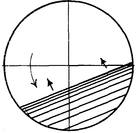
Fig.7 Spiral Scan ground return reference
If a gate circuit is set up
which permits signals to pass only
when the applied potential is equal
to a given value, then the Y plate
signal may be applied to this gate
and the trace brightened up only
at a specified line below the centre
of the tube, e.g. fig. 8.
A suitable gate circuit is the
long tail pair. The input to the
left-hand grid is the time base
sine wave from the Y plate and a
level is set up on the
movement right-hand grid; shifting this
potential alters the
height at which the
straight line appears
on the tube.
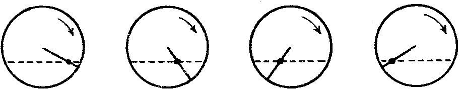
Fig.8 Locus of point
So that the lines may remain straight and yet rotate about the tube centre, instead of taking the Y potential for matching to the gate potential, X and Y resolution is employed and sine and cosine voltages obtained from X and Y plates. These are combined in a magslip (X potentials being fed to one stator and Y potentials to the other) and the resultant obtained from the rotor. This is applied to one grid of the long tail pair and on the other grid is fed a voltage developed across a resistance, varied mechanically in synchronism with the scanner. This produces a voltage change for every scanner revolution to simulate the actual law followed by the ground returns. In addition, a fraction of the voltage proportional to the height of the synthetic aircraft (obtained elsewhere in the trainer) is mixed with this signal to obtain "climb and dive" appearance of the synthetic ground return. A diagram of the arrangement is given below. (Fig.9)
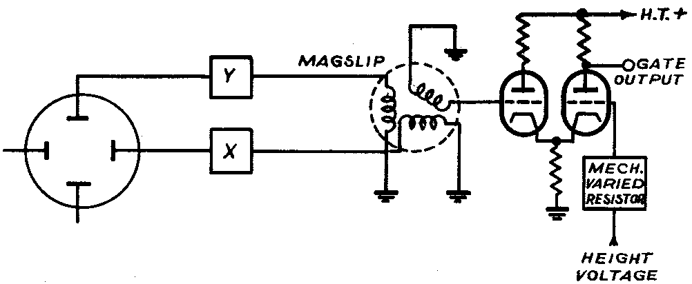
Fig.9 Gate circuit for simulation of spiral scan ground returns
(d) Gate Circuit
for Target and
Beam Co-
incidence
Most of the
recent AI equipments
use a range/azimuth
presentation.
Relative elevation
is sometimes displayed on the same
tube by the double dot method and sometimes on a separate
tube. The target echo is shown as an intensity modulated
spot when the narrow beamed pulses are reflected. To simulate
the coincidence of the scanner beam with the target, with bank
and pitch of interceptor taken into account, the following
circuit has been used. (See Fig.10)
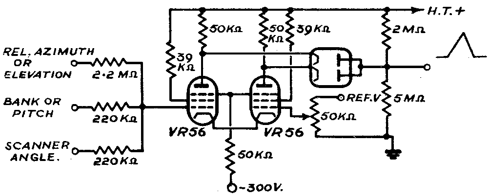
Figure 10. Gate circuit for target and beam
coincidence
On one valve of a long tailed pair the control grid is taken to a reference voltage, the control grid of the other being fed from a network containing potentials due to:-
With no bank, scanner dead ahead and relative azimuth or
elevation angle zero the potentials for the network are equal
to the reference voltage and the anode voltages are equal.
A change of any of these functions results in unbalance and
one anode rises whilst the other falls. This unbalance due
to the change of one of the functions can be compensated by a
change of one of the others, thus restoring the anodes to
balance. By coupling the cathodes of a double diode one to
each anode and the diode anodes together to a high impedance
potential divider, the common diode anode follows the lower
potential LTP anode on either side of the balance potential.
This "peaking" voltage is used to control the amplitude of a
-suitable pulse at the target range.
(e) The 360° Continuous Potentiometer System
Mention should be made of an all-round continuous
potentiometer system which is used for remote control purposes.
The two potentiometers each consist of a continuous toroidal
resistance element tapped at four points 90° apart, and having
two separate sliders diametrically opposite each other. (See
Fig.11). The two potentiometers, master and slave, have their
four taps connected together in order and a voltage is applied
across the sliders of the master potentiometer. No voltage
appear across the sliders of the slave potentiometer
when they are electrically at right angles to those of the
raster potentiometer. Any variation from this position produces a positive or negative voltage across the sliders which
is amplified and fed to a servo-motor system. This rotates
the slave potentiometer shaft in the correct direction for
rebalance so that rotation of the master potentiometer is
immediately followed by rotation of the slave potentiometer,
continuously over 360°. By using four tappings, which is the
minimum number for theoretically perfect following, the
limiting accuracy is determined by the pitch and linearity of
the winding and the geometrical accuracy of the sliders and
tappings. These potentiometers are made in two types, one
with fixed body and one with a rotatable body which can be
used in an rθ calculator described in para. 5(a).
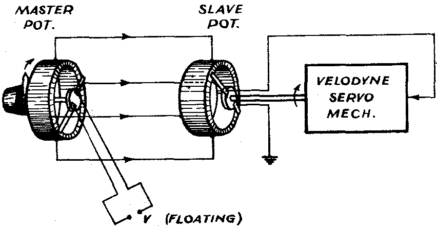
Fig. 11 360° Continuous Potentiometer System
5. CONTROL OF MOVING SYNTHETIC TARGETS IN TWO DIMENSIONS
(a) rθ Polar Co-ordinates Calculator
For the production of tracks representing the plan movement of an aircraft it is necessary to calculate changing
ranges and bearings of the target as seen from the home
station. Information to the calculator is provided in the
form of aircraft course, rate of turn and speed, and the
output required is Range and Bearing.
Let Ø = Bearing of aircraft from station
Ω = Course of Aircraft
Rp = Plan range (in this case taken to be equal to slant
range as the angle of elevation is extremely small)
(also assumed by ground PPI's)
V = ground speed of aircraft
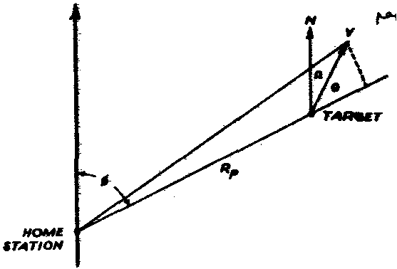
Fig.12 Co-ordinates of moving target from fixed station
From the diagram (fig.12) it
will be seen that
dRp/dt = V cos 8 - where θ = Ø - Ω
dØ/dt = (V sin θ)/Rp
The subtraction of Ø - Ω is
carried out by the use of a
360° potentiometer where Ø is
an angular rotation of the
body of the potentiometer
equal to bearing, and Ω is
the rotation of the slider of
the potentiometer (controlled by servo mechanism from a link
:trainer or synthetic flying unit) equal to aircraft course.
This angle θ is transferred to a sine law potentiometer which
is energised by a voltage V proportional to speed. From the
sliders of the potentiometer the quantities V cos θ and
V sin θ are obtained. V cos θ is integrated by a Velodyne
integrator to give the result Rp as the rotation of the
sliders of a two-gang potentiometer. One slider gives Rp as
a voltage. The other potentiometer is used to perform the
operation of dividing V sine θ by Rp. This voltage ((Vsinθ/Rp)
is integrated by a second Velodyne whose output rotates the
body of the 360° potentiometer previously mentioned and also
the gating circuit as described in paragraph 2(b). Continuous
range and bearing are thus obtained as shaft rotations, which
may be geared down and used to drive range and bearing
potentiometers, or dials, as desired.
(b) Photo-cell and Film Technique
Figure 13 Photo-cell and film technique
Tracks may be controlled in range and bearing by the
method outlined in fig.13. The time base of the Plan Position
Indicator is duplicated
(but non-rotating) on a
smaller high actinic tube
of great brilliancy. A
roll of black paper is
moved across the tube face
at a speed. synchronised
to the rotation of the
time-base. Each frame
then represents one
revolution of the PPI and distance along the frame
can represent bearing in
degrees. Range is
proportional to the distance across the frame,
therefore if holes are punched in each frame, differing
slightly in range and bearing from frame to frame, simulation
of moving echoes can be obtained. The photo-cell collects
the light projected through the hole and the voltage pulses
produced are amplified and applied to the PPI tube as intensity
modulation. It is possible, by a development of this system
now in the research stage, to photograph any PPI or moving
presentation and reproduce it at a later date on a synthetic
trainer.
(c) Walking Crab System
A small synchronous clock motor is arranged to drive a
crab round a fixed point on a table, this point representing
the home station (see fig. 14). The direction of motion of
the crab is set by
a "course" knob
on the crab.
Fig. 14 Moving Crab System potentiometer
Speed is controlled by feeding the motor from a variable frequency oscillator. A link arm turns a potentiometer for control of bearing and a string fixed to the crab pin (representing aircraft) draws a spring loaded potentiometer round to give a potential for control of range. A small pencil mounted underneath the crab below the pin, records the track covered. This is probably the simplest method of obtaining two dimension tracks.
(d) Ultrasonics Technique
This technique has proved one of the most successful
the design of trainers for simulating ground tracks as seen
by radar from a loving aircraft, e.g., H2S, ASV, etc.
This miniature radar system employs ultrasonic waves propagated in water. A 13.5 Mc/s crystal under water is pulsed at the same recurrence frequency and pulse length as the radar equipment it is simulating.
Since the velocity of ultrasonic waves in water is 1.5x
105 cm/sec. and that of electromagnetic waves in air is
3 x 1010 cm. per sec. the trainer scale is
(1.5 x 10⁵)/(3 x 1010) = 1/200,000of the radar scale
i.e. one ultrasonic mile = .315 inches and a radar range of
50 miles can be encompassed in a physical distance of 15".
At a frequency of 13.5 Mc/s, with a velocity of 1.5 x
105 cm/sec.
λ = (1.5 x 10⁵)/(13.5 x 106) = 0.1 mm.
With a crystal of 5 mm x 25 mm, this is equivalent to an
aerial array of 50λ x 250λ. The beam is thus quite sharp
and rectangular.
The crystal beam is projected on to a glass relief map so that to projection covers a range of 0-30 miles (0-10 ins. approx.) The map is sand-blasted to represent land masses, while rivers and sea areas are left polished. Towns are built up in granules of carborundum. The pulsed crystal is rotated at the same speed as the aircraft scanner. H2S or ASV scanning is therefore simulated and a synthetic picture is built up. If the scanning crystal is mounted on a gantry it can move over the relief map for navigation training. A duplicate plotting map (not relief) is mounted above the crystal assembly and a recording pen on the crystal assembly marks the under side of the plotting map to record the flight of the synthetic aircraft. Complete crew training is achieved with pilot flying a link trainer under the H2S or ASV operator's instructions. The operator sees a continuous change of picture as the synthetic aircraft "flies" over the target area.
6. CONTROL OF MOVING SYNTHETIC TARGETS IN THREE DIMENSIONS
(a) Fundamental Problems
The fundamental problem is the representation continuously changing vectors in three dimensions for two
aircraft in still air. For radar AI systems the final aim
of an AI trainer is to give the pilot and operator as nearly
as possible the actual experience of an AI interception.
An AI night combat can be represented in four-stages, the GCI
vector, the AI chase, the visual contact and the moment of
firing.
A synthetic AI trainer must therefore consist of the following:-
The changing movements of two aircraft in space which
must be taken into account in trainer design are:-
AI Equipped Fighter Enemy Bomber Enemy Bomber
1. Fighter's changes in course. 6. Bomber's changes in
2. Fighter's changes in height. course. 7. Bomber's changes in height.
3. Fighter's changes in air
speed 8. Bomber's changes in air speed
4. Fighter's banking movements. 9. Bomber's banking movements
5. Fighter's pitching movements. 10. Bomber's pitching
movements
11. Absolute bearing of bomber from fighter.
12. Absolute elevation of bomber from fighter.
13. Range between the two planes.
(b) Electrical
Representation
of Co-ordinates
 A D.C. system which
was developed at TRE,
but which has now been
superseded by an A.C. Continuous Calculator,
is mentioned for
interest. This system
A D.C. system which
was developed at TRE,
but which has now been
superseded by an A.C. Continuous Calculator,
is mentioned for
interest. This system
arbitrarily represents
values of heights,
courses, speeds, etc.,
as voltages.
A course of due north can be arbitrarily represented by a potential of 150 volts, N.W. by 280 volts and N.E. by 30 volts. A height of 20,000 ft. can be represented as 280 volts and 500 feet as 30 volts (these figures being consistent with normal valve characteristics). A 300 volt negative supply is used to obtain voltages representing bomber's actions and a 300 volt positive supply for fighter's actions. This is shown in fig.15, where two aircraft are represented as flying in different directions.
The course difference Fig.15 Electrical representation between the two planes is of co-ordinates obtained by simple subtraction of voltages. At a range of 20,000 ft. a certain course difference will produce 1/40th of the effect of an equal course difference at 500 ft. Course difference, therefore, must be divided by range and integrated to give the absolute bearing between the two aircraft. This potential can be fed to the grid of one valve of a long tail pair and a potential representing the fighter course to the other, and the difference appearing at the anode can be used to control the AI indications in azimuth.
Elevation indications can be obtained in the same manner, e.g." fighter pitching movements control a potential and can be termed rate of climb, (or dive). This is integrated as height and is a positive potential. The Bomber (negative) potential is subtracted and when this potential difference is zero both aircraft are taken to be at the same height. The height difference potential divided approximately by range is fed to one grid of a long tail pair and the other is connected to the fighter pitch potential. The difference potential appearing at the anode then represents relative elevation.
The effect of fighter bank on the Al presentation is to rotate the picture as a whole, and this is effected by making use of the rotational effect of a magnetic focusing coil, or by rotation of magslips as described in 4(c). Standard 10 mA FSD milliammeters, fed from cathode followers, can be arranged to move in a fashion similar to the instruments on a normal aircraft blind flying panel.
(c) Air to Air Continuous Calculator
In the design of this calculator the motions of the two
synthetic aircraft in azimuth are separated from the motions in elevation, being combined in a later stage to give slant
range. Referring to the diagram fig. 16.
Fig. 16 A.C. 360° Continuous Calculator
Let Ωf = friendly course.
Ø = bearing between friend and enemy
Ωe = enemy course
Rp = plan range
Vf = resolved velocity of friend in horizontal plane
Ve = resolved velocity of enemy in horizontal pane.
Then the relative azimuth of enemy to friend is Ø - 2f.
If the velocities of friend and enemy are resolved at right
angles to the line of join (or Rp), the rate at which the
bearing of the enemy is changing is given by:-
dØ/dt = (Vf sin (Ø - Ωf) -Ve sin (Ø - Ωe) / Rp
and the rate of change of range:-.
dRp/dt = Vf cos (Ø - Ωf) - Ve cos (Ø - Ωe)
These expressions are integrated to give bearing and
range. Slant range and angle of elevation are obtained from
plan range and height difference and the triangle solved by
magslips, as described below.
Let Δ = angle of elevation
Hf = height of friendly plane
He = height of enemy plane
Rp = plan range
Rs = slant range
Rv = vertical range
then tan Δ = (Hf -He) / Rp = Rv / Rp (see fig, 17)
Fig.17 Elevation Calculation
Feeding in Rv and Rp the calculator is required to produce Δ and Rs.
The complete system of the continuous calculator is as follows:-
A master oscillator (RC type) operating at 2000 cycles feeds two cathode followers. One of the cathode followers is coupled to the rotor of a small magslip representing Friendly course. The other feeds the rotor of a magslip representing Enemy course. The secondaries are joined in series and, if the stators are rotated by an amount proportional to Ø, the amplitudes of the resultant A.C. voltages in X and Y planes are proportional to:-
Vf sin (Ø - ΩF) )
Ff cos (Ø - ΩF) ) on friendly course magslipVe sin (Ø - ΩE) )
Ve cos (Ø - ΩE) ) on enemy course magslip
A phase discriminator determines the sign of the function
in each case and switches the "sense" of the velodyne
integrator accordingly. The phase discriminator operates
on the principle of the master sine wave acting as HT on a valve with the input wave fed to the grit. No anode current
is passed unless both are in phase. The sine function of
the magslips is fed to a resistance, the correct voltage
being tapped off according to the correct law for "divide by
range". Across the slider of the resistance is therefore:-
(Vf sin (Ø - ΩF) - Ve sin (Ø - ΩE)) / Rp
This is integrated by a linear velodyne integrator and appears
as a rotation of shaft for bearing. The cosine function from
the other pair of stators is also phase discriminated similarly
and fed to a linear integrator to provide plan range. The
input to this integrator is:-
Vf cos (Ø - ΩF) - Ve cos (Ø - ΩE)
This shaft is used to control the "divide by Range"
mechanism on the bearing integrator.
Elevation is obtained by solving the triangle. Rp, Rs and Rv (see fig. 17). A magslip with two rotor windings is used. An A.C. potential proportional to plan range (from Range Velodyne) is fed to one stator. Height difference between the two planes is obtained by means of a differential into which is fed the friendly and enemy height as shaft rotations. An A.C. potential proportional to height difference is fed to the other magslip stator. The resultant of the two fields is now the third side of the triangle. If the magslip rotor is turned until there are no volts induced in its windings, then it is at right angles to this resultant. This "null" method is more accurate than a "max" method and is automatically controlled by a further Velodyne. The second rotor winding is at right angles to the first and will therefore be in a position of maximum field and the voltage induced in it is the resultant of Rp and Rv, i.e., slant range. This voltage is rectified and used for controlling the presentation. Absolute elevation is derived from rotation of the magslip shaft and subtracted from the pitch angle obtained from the flying unit.
(d) Visual Target Presentation
In the design of AI trainers it is essential that for
complete crew training the four requirements mentioned in 6(a)
should be fully met and therefore it is necessary to project
on a screen ahead of the pilot an image of the enemy bomber
under correct night illumination conditions so that the change-over between the AI chase and visual contact can be made.
Fig.18 Optical System of Target Projection
Fig. 18 shows a system of moving lenses which has been designed to provide this effect. The lenses (a) and (b) are cam operated so that their motions give variable sizes of the image without loss of focus so that the image size is inversely proportional to the range between the two planes. The background illumination representing full moon, half moon, starlight, etc., from lantern A is photometrically matched with the illumination from lantern B (illuminating a model bomber) in a 1/32 inch hole cut in the centre of the mirror M which is inclined at 45° to the optic axis. The matched picture is projected into the plane of a sky slide, which is moved vertically and horizontally by Servo motors to obtain the motion of the enemy aircraft relative to the sky. By means of a second lens this picture is moved vertically and horizontally in accordance with relative motions between fighter and bomber aircraft. The whole picture is then rotated by an erecting prism controlled by Servo motors from the banking motions of the fighter. An accurate scale model of 1" = 100 ft. of an enemy bomber is mounted in perspex on gimbals and is capable of rotation in four movements, enemy bank, course, pitch and "aspect" (i.e. when approached by the fighter from above or below) all movements being controlled by Servo motors from a small joy stick on the instructor's unit. The enemy aircraft can thus be "flown" to represent the enemy taking evasive action.
(e) Synthetic Flying Units
In all AI trainers the pilot and AI operator should be
trained as a team. The operator, from his picture on the
tube, instructs the pilot to climb, turn, increase or decrease
speed, etc., which in turn, alters the operator's picture.
In early trainers a simple flying unit was devised, but units
designed on correct aerodynamical lines have become essential if the correct flying and operating techniques are to be
carried out.
In the early types of flying unit a simple mock-up of
the pilot's position was used with the joy stick, throttle,
etc.; controlling potentiometers over limited degrees of
travel. The blind flying instruments consisted of 0-10 mA
meters, suitably calibrated as Air Speed Indicator,
altimeter, artificial horizon, turn and bank indicator, etc.
This was used with the "limited angle" calculator described
in 6(b).
The final flying unit has been designed to give correct "fuel of controls" and to fly aerodynamically as nearly as
it is possible to "fly" on a ground trainer. Three sets of
axes have been taken into account (see diagrams, fig.19).
Fig.19 Axes relative to earth, aircraft, and line of
flight.
The aerodynamical terms are defined as follows:-
L = Lift = IPV2 x CL x S Where p = air density
S wing area
CL = coefficient of lift
D = Drag = z pV2 x CD x S Where CD = coefficient of drag
W = weight
V = air speed
T = engine thrust
Six computors are used to calculate the following:-
(1) Bank is calculated from the following terms
(a) Aileron angle
(b) Rate of turn
(c) Rudder angle
(d) A stability term, due to side slip
(2) Angle of Incidence from terms representing
(a) angle of elevator
(b) thrust
(3) Angle of Climb from terms representing
(a) lift
(b) weight
(c) engine effect (due to change in angle of incidence)
(d) Rudder effect on climb
(4) Aircraft Course from terms representing
(a) Rudder effect
(b) Lift
(c) Engine effect (due to change in angle of yaw)
(5) Aircraft Speed from terms representing
(a) Engine thrust
(h) Drag
(c) Weight (Groundspeed is also calculated (V cos θ))
(6) Aircraft Height from
(a) Rate of Climb
The synthetic flying unit has been designed to simulate the aerodynamic characteristics of a "Mosquito" aircraft. The mock-up fuselage is fitted with standard Mosquito control column, rudder bar, throttle, trimmers, etc., and the original set of blind flying instruments are modified to operate from the trainer.
The "feel of controls' effect is obtained by straining (in the case of aileron or rudder) against suitably placed springs. In the case of elevator pressure is exerted against a servo- mechanism which is fed with a voltage proportional to elevator hinge moment. As the aerodynamic characteristics of any aircraft are known it is possible to change the resistances representing aircraft quantities and the lift and drag cams, to simulate other types of aircraft.
(f) Relative Motion Indicators
In the design of trainers for centimetre equipment
(particularly AI) a light beam can be used to simulate the
narrow cm beam and a photo-cell to represent the enemy plane.
The light beam is made to scan in a similar fashion to the
radar scan it is simulating and the photo-cell can be
automatically moved by servo-motors in the scan to simulate
the enemy's movements. For a trainer simulating AI Mark 8 a
mechanical device has been designed to produce the spiral scan
by a light beam. Voltages proportional to relative elevation
and relative azimuth of the two synthetic planes from the
flying unit are fed to Velodyne servo systems which control
the position of the photo-cell. As the two synthetic planes
change positions in space the photo-cell automatically takes
up the correct position to give the changing presentation to the operator. A diagram of the mechanical device is given
below (Fig.20). These mechanical devices are known as
Relative Motion Indicators, and other types have been designed
for other marks of AI.
Fig.20 Relative Motion Indicator
CONCLUSION
It has not been possible, in the space of this Journal, to
give full details of design, but it is hoped that the
broad outlines of the techniques used in trainer design may
be of interest. Further information on the circuits described may be found in the reports issued by the Trainer
Design Group. Two of the subjects, Continuous Calculator
design and Ultrasonics techniques, are to be dealt with at
greater length in a future TRE Journal.